OWS Styling HOW-TO Guide: Colour Map Styles
Colour Maps
Discrete measurement bands (i.e. bit-flag or enumeration bands) demand very different visualisation approaches than continuous measurement bands, and they are not well served by the sorts of component and ramp based styles we have discussed so far [1].
Example Data
A good example of a discrete data band from the Digital Earth Australia archive is the daily Landsat Water Observations from Space (WOfS) product. (I use the newer “Collection 3” release here.)
This sample data is from the northern coast of Australia, on the border between WA and NT, on Christmas Day 2020 and yields a 1038 by 815 pixel image:
from datacube import Datacube
dc = Datacube()

wofs_data = dc.load(
    product='ga_ls_wo_3',
    measurements=['water'],
    latitude=(-15.9098, -15.0496),
    longitude=(128.0882, 129.2171),
    time=('2020-12-24T10:00:00', '2020-12-25T09:59:59'),
    output_crs="EPSG:3577",
    resolution=(-120,120),
    group_by="solar_day"
)
The WOfS “water” band is a bitflag band. The available bitflags can be viewed by inspecting the
product metadata (e.g. with datacube product show ga_ls_wo_3). The relevant extract of the
metadata is shown below (YAML format).
measurements:
  - name: water
    flags_definition:
      nodata:
        bits: 0
        description: No data
        values: {0: false, 1: true}
      noncontiguous:
        bits: 1
        description: At least one EO band is missing or saturated
        values: {0: false, 1: true}
      low_solar_angle:
        bits: 2
        description: Low solar incidence angle
        values: {0: false, 1: true}
      terrain_shadow:
        bits: 3
        description: Terrain shadow
        values: {0: false, 1: true}
      high_slope:
        bits: 4
        description: High slope
        values: {0: false, 1: true}
      cloud_shadow:
        bits: 5
        description: Cloud shadow
        values: {0: false, 1: true}
      cloud:
        bits: 6
        description: Cloudy
        values: {0: false, 1: true}
      water_observed:
        bits: 7
        description: Classified as water by the decision tree
        values: {0: false, 1: true}
Example: Simple Flag-Based Colour Map
Colour Maps work on a single band by defining a series of logical rules, with the first rule a pixel matches determining the colour of the pixel. Let’s start with a simple example:
simple_map_cfg = {
    "value_map": {
        # Value_map maps a band to a list of rules.
        # Do not put multiple bands with independent rules into a single value_map. It
        # may appear to work, but in practice you cannot guarantee which band will be checked
        # for matches first, and therefore the output may render inconsistently from one python
        # instance to another.
        "water": [
            {
                "title": "Water",
                "abstract": "",
                "flags": {"water_observed": True},
                "color": "Aqua",
            },
            {
                "title": "Cloud",
                "abstract": "",
                "flags": {"cloud": True},
                "color": "Beige",
            },
            {
                "title": "Terrain",
                "abstract": "",
                # Flag rules can contain an "or" - they match if either of the conditions hold.
                "flags": {"or": {"terrain_shadow": True, "high_slope": True}},
                "color": "SlateGray",
            },
            {
                "title": "Cloud Shadow and High Slope",
                "abstract": "",
                # Flag rules can contain an "and" - they match if all of the conditions hold.
                "flags": {"and": {"cloud_shadow": True, "high_slope": True}},
                "color": "DarkKhaki",
            },
            {
                "title": "Dry",
                "abstract": "",
                "flags": {"water_observed": False},
                "color": "Brown",
            },
        ]
    }
}
The results look like this:
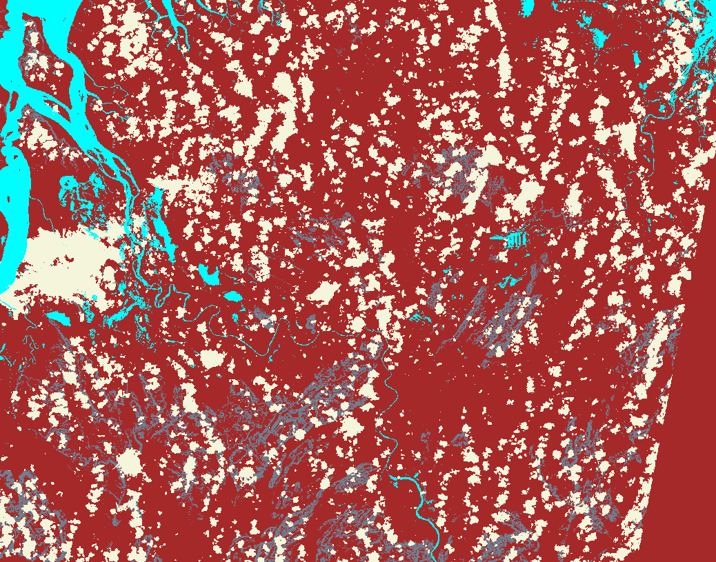
This all looks a bit of a mess. The problem is that rules are evaluated in order, which can result in unexpected behaviour if you are not paying attention.
Issues include:
The “Terrain” rule matches all pixels with the high_slope bit set, so the “Cloud Shadow and High Slope” rule can NEVER be triggered.
The water observed flag is matched early, so false-positive water observations from cloud pixels can occur.
Example: Better Flag-Based Colour Map
Let’s construct a better ordering:
better_map_cfg = {
    "name": "observations",
    "title": "Observations",
    "abstract": "Observations",
    "value_map": {
        "water": [
            # Cloudy Slopes rule needs to come before the Cloud
            # and High Slopes rules.
            {
                "title": "Cloudy Slopes",
                "abstract": "",
                "flags": {"and": {"cloud": True, "high_slope": True}},
                "color": "BurlyWood",
            },
            # Only matches non-cloudy high-slopes.
            {
                "title": "High Slopes",
                "abstract": "",
                "flags": {"high_slope": True},
                "color": "Brown",
            },
            {
                "title": "Cloud",
                "abstract": "",
                "flags": {"cloud": True},
                "color": "Beige",
            },
            {
                "title": "Cloud Shadow",
                "abstract": "",
                "flags": {"cloud_shadow": True},
                "color": "SlateGray",
            },
            # Match water AFTER special pixels.
            {
                "title": "Water",
                "abstract": "",
                "flags": {"water_observed": True},
                "color": "Aqua",
            },
            {
                "title": "Dry",
                "abstract": "",
                "flags": {"water_observed": False},
                "color": "SaddleBrown",
            },
        ]
    }
}
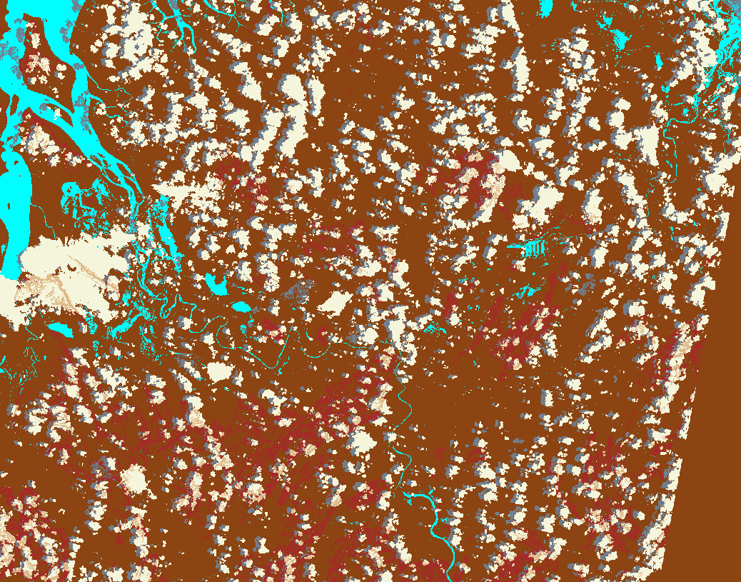
Note the differences coming from the order in which the rules are evaluated.
Example - Transparency Rules
In the bottom right corner we can see a wedge of pixels that is obviously outside the satellite path, but is being coloured “Dry”. We really should make these pixels another colour, and ideally transparent.
There are two ways we can get transparent pixels in colour
maps. Firstly, we can use an alpha element beside color. This ranges from 0.0 (fully
transparent) to 1.0 (fully opaque, the default), as for colour ramp styles.
Secondly, all pixels that do not match any rules default to being transparent.
transparency_map_cfg = {
    "value_map": {
        "water": [
            {
                # Make noncontiguous and invalid data transparent
                "title": "",
                "flags": {
                    "or": {
                        "noncontiguous": True,
                        "nodata": True,
                    },
                },
                "alpha": 0.0,
                "color": "#ffffff",
            },
            {
                "title": "Cloudy Steep Terrain",
                "flags": {
                    "and": {
                        "high_slope": True,
                        "cloud": True
                    }
                },
                "color": "#f2dcb4",
            },
            {
                "title": "Cloudy Water",
                "flags": {
                    "and": {
                        "water_observed": True,
                        "cloud": True
                    }
                },
                "color": "#bad4f2",
            },
            {
                "title": "Shaded Water",
                "flags": {
                    "and": {
                        "water_observed": True,
                        "cloud_shadow": True
                    }
                },
                "color": "#335277",
            },
            {
                "title": "Cloud",
                "flags": {"cloud": True},
                "color": "#c2c1c0",
            },
            {
                "title": "Cloud Shadow",
                "flags": {"cloud_shadow": True},
                "color": "#4b4b37",
            },
            {
                "title": "Terrain Shadow or Low Sun Angle",
                "flags": {
                    "or": {
                        "terrain_shadow": True,
                        "low_solar_angle": True
                    },
                },
                "color": "#2f2922",
            },
            {
                "title": "Steep Terrain",
                "abstract": "",
                "flags": {"high_slope": True},
                "color": "#776857",
            },
            {
                "title": "Water",
                "abstract": "",
                "flags": {"water_observed": True},
                "color": "#4f81bd",
            },
            {
                "title": "Dry",
                "abstract": "",
                "flags": {"water_observed": False},
                "color": "#96966e",
            },
        ]
    },
}
As with the Colour Ramp examples already seen, transparency is declared with and “alpha” value ranging from 0.0 (fully transparent) to 1.0 (fully opaque). You must define a colour, even if alpha is zero. Alpha is optional and defaults to 1.0 (fully opaque).
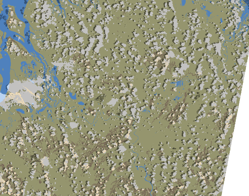
The clouds are clearly visible, with only the separately derived terrain data and the noisy water-detection bits visible through the cloud, with clearly defined cloud shadows and clear water detection.
Enumeration Bands
Sometimes you may have a band that contains an enumeration code value rather than a bitflag. In this case we can use a “values” rule instead of a “flags” rule, where we explicitly specify all the matching values.
E.g. because for wofs if the “nodata” is set then other bit can be set, the following are equivalent:
# Using a "flags" rule.
{
    # Make noncontiguous and invalid data transparent
    "title": "",
    "abstract": "",
    "flags": {
        "nodata": True,
    },
    "alpha": 0.0,
    "color": "#ffffff",
},

# Using a "values" rule.
{
    # Make noncontiguous and invalid data transparent
    "title": "",
    "abstract": "",
    "values": [
        1,    # nodata
    ],
    "alpha": 0.0,
    "color": "#ffffff",
},
We’ve seen how to use transparency in colour-ramp styles in the last chapter, and in colour-map styles in this one. In the next chapter we explore other ways of achieving transparency in datacube-ows.